Golden Snake: Summer of Math Exposition 2

“Life lies in movement.” — Voltaire

Summer of Math Exposition 2

3Blue1Brown, a well-known math YouTuber, is hosting the Summer of Math Exposition 2 (SoME2), a math lesson competition in which anybody in the world can submit a video or blog post which teaches the audience a lesson in math. Last year, I missed out on the opportunity to participate, so I will be taking the chance this time around. I would have liked to make a video, but that simply takes up too much time.

Introduction

Have you ever checked your answer sheet during a test and found 3 or 4 repeated answers? It’s not a great feeling. Even though we may know the material well, that type of pattern showing up in what should be a random spread of answers tends to create some doubt.

“Random,” a word that our modern culture has taken to mean “weird” and “unpredictable,” actually describes something that creates predictable trends in the long term.

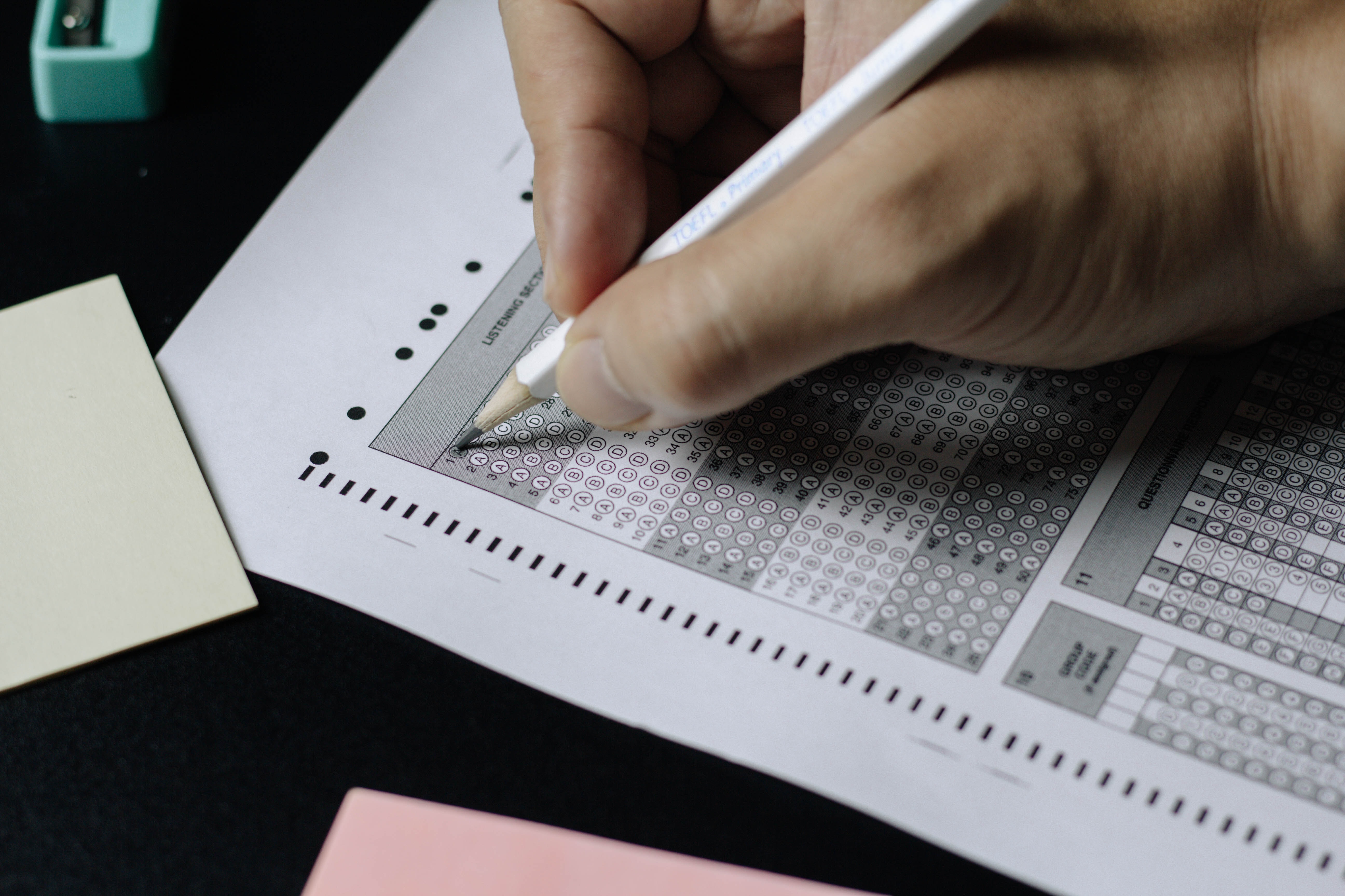Credit to Nguyen Dang Hoang Nhu

Proof?

Don’t believe me? Let’s take the example of flipping a coin on heads 3 times in a row. We know that the probability of this is $(\frac{1}2)^3$, or one-eighth. But, as for the actual outcome of one trial, we don’t really know what will happen since there is a lot of variability.

However, if we repeat this process $1000$ times, we can be quite sure that the number of successes will be $\approx 125$.

The Problem

Have you ever filled out a multiple-choice answer sheet and tried to look for patterns in the answer order to see if you got anything wrong? For instance, if you get four of the same choice in a row, you might want to reconsider.

In this video, we will look at the probability of getting the pattern of a snake, given random answers on a test with $10$ questions, $4$ choices each.

There is only one rule for a snake: the next answer must be at most one away from the current answer. If we start on A, the next answer must be A or B. If we start on B, the next answer can be any letter except for D.

Some Vocabulary

I will refer to questions as rows, since they go horizontally from left to right, and instead of saying ABCD, I will sometimes say column 1234, since they go up and down vertically. And for each answer and row combination, I might refer to it as a cell instead, as in a cell in a spreadsheet.

Brute-force Listing

Firstly, we can just try to list the number of ways that each row can have a snake end on it.

So, it would be $1+1+1+1=4$ for the first row, $2+3+3+2=10$ for the second row, and $5+8+8+5=26$ for the third, $13+21+21+13=68$ for the fourth.

Finding Patterns

Generally, we should be able to see some patterns in the first couple of rows.

Mirroring

I notice that there is mirroring between the left and right halves of every row.

This means that we are actually storing more information than we need to, since the results can actually be predicted from just the left or right side of the sheet.

The total sum for each row should be $2(A+B)$, since $A=D$ and $B=C$.

Contributions

For every A cell after the first row, the contributions of the previous row to it will be $A+B$. For every B cell after the first row, the contributions of the previous row to it will be $A+B+C$, which is really just $A+2B$ due to mirroring.

Sequential patterns

Avid math fans may already notice a certain sequence appearing somewhere, but we will be saving it for later, since it would not be fun to reveal it now.

Let’s look at the totals for each row, $4, 10, 26, 68$. At first, these numbers seem to not be related at all, but we can always try to look at the differences between each subsequent pair. We get $6, 16, 42$. This still looks kind of strange, so let’s do that again. We get $10, 26$.

Now, I’m starting to see a similarity between this sequence and the original totals. $10, 26$ appear in both, and we can verify that is not a coincidence by extending the original sequence.

However, why does it only begin to match up on the second number in the first sequence, and not the first?

Let’s try to look for a pattern that involves the sequences, but within the columns:

• Sequence 1: $4, 10, 26, 68…$
• Sequence 2: $6, 16, 42, 110…$
• Sequence 3: $10, 26, 68, 178…$

To me, it seems like the nth element of Sequence 3 is just the sum of the nth elements of Sequence 1 and 2. For now, let us assume that this is true without going into why exactly it is true.

Differences, Differences, Differences

But, what does this equality really mean?

Well, remember that Sequence 2 is actually the differences, also known as the rates of change, of the original sequence. As such, Sequence 3 is the rate of change of the rate of change of the original sequence.

So, what we are saying is that the sum of Sequence 1 and its rate of change is equal to Sequence 1’s rate of change’s rate of change.

Differential Equations

If we write this in the language of calculus, we end up with the differential equation, $y+y’=y’’$

While I will not explain all of the details, we will assume $y=f(x)$ is of the form $y=e^{mx}$. This then allows us to get the equation $m^2-m-1=0$, which we can solve with the quadratic equation.

$m=\frac{1+\sqrt{5}}2, \frac{1-\sqrt{5}}2$

By the way, these numbers are known as $\phi$ and $1-\phi$, this will be important later, but you’ll just need to be patient.

So, we have two solutions to our differential equation: $e^{\frac{1+\sqrt{5}}2x}$ and $e^{\frac{1-\sqrt{5}}2x}$. Since we had a homogeneous linear differential equation, we can use any linear combination of solutions to make a new solution. This means that $y=Ae^{\frac{1+\sqrt{5}}2x}+Be^{\frac{1-\sqrt{5}}2x}$

To solve for A and B we can use the initial values of $y(0)=4, y’(0)=6$ to create a system of equations.

Small Issue

Now, we do get valid results. If we try to find the x values at which our first sequence’s values appear, they are roughly spaced equally apart. However, the spacing is not 1, but some changing amount around $0.59$. This will not do: if we do not know how to get the next number in the sequence, we simply have not solved the problem.

But, why does our solution not work? Well, we came up with three discrete sequences, where the differences are actually instantaneous rates of change that are also applied instantaneously. However, the total change after a change of 1 in x will be greater than our instantaneous rate of change, since our rate of change increases the whole time.

So, how can we fit a line to our data if our differential equation does not work? By the way, the problem is not the initial value, even if we have $y(0)=4$ and $y(1)=10$, the differential equation will still be incorrect, since we already start with the wrong $y’(0)$ that doesn’t line up with our sequence, as the only way to have $y’(0)=6$ is incorrect.

As long as we maintain this rule that only works for discrete sequences, we will have no success in the continuous sense. So, let’s try a different approach.

Concluding Diff-scussion

While I have no idea how to make the differential equation work for the problem, the format of the differential equation solutions is very interesting, and may give us a clue for the eventual solution…

Matrix Method

We’ve structured our problem into a grid of numbers, so the natural question to ask is, “Will matrices help us?”

Matrices are rectangular grids of numbers denoted with square brackets on the left and right, they function like groups of numbers.

One of the most common operations for matrices is matrix multiplication. In short, when two matrices are multiplied, the result is a matrix filled with the sums of the products of the rows of the left matrix and the columns of the right matrix.

Here is a video teaching you how it works from ya boi, Organic Chemistry Tutor:

An important note here is that the left matrix’s number of columns must equal the right matrix’s rows.

Applying Matrix Multiplication

For this section, you may want to check out 3B1B’s videos on how matrix multiplications are like applying transformations:

Perhaps there is a way to store the combinations for each column at a given row within a matrix, let’s call this our original matrix, then multiply it by some other matrix on the left, let’s call it a scaling matrix, to get to the values for the combinations of the next row!

So, what will be our original matrix and what will be our scaling matrix?

Shall we have $\begin{bmatrix}1 & 1 & 1 & 1\end{bmatrix}$ as our original matrix? After some thought, this would probably not work out, since we would only be able to multiply each column’s value by a single number, and that is not enough to create the complex pattern of combining multiple columns’s information into one through addition.

Scaling Matrix

Perhaps, it would be easier to start with the scaling matrix on the left.

Before starting to ask how we can sum the values from multiple columns, let us ask how we can at least keep the original matrix the same.

Identity Matrix

This is akin to asking, for scalar multiplication, “What number do we multiply x by to keep it the same?”

This may come as a shock to some of you, but the answer is 1. How do we apply this to matrix multiplication though?

When we do matrix multiplication, the output matrix is computed in the order that we read books, from left to right, then from up to down. When we multiply, while we do look at the right matrix from left to right, the entire column is included in the operation. However, within this column, we only want one number to be in the output, the number in the current row.

Of course, we just want to multiply this number by one and multiply the other numbers in the column by zero so that we can move onto the next column. To do this, we need the left matrix to have a one somewhere, and zeroes in the rest of the row. Where shall we put it?

For the first row of the left matrix, we should place the one in the first place, so that it can multiply with the all the numbers in the first row of the right matrix. For the second row, we should place the one in the second place for a similar reason.

So, we end up with this neat pattern, a square with ones on the diagonal, zeroes everywhere else. We know this as the identity matrix and, therefore, the starting point of our scaling matrix.

$\begin{bmatrix} 1 & 0 & 0 & 0\\ 0 & 1 & 0 & 0 \\ 0 & 0 & 1 & 0\\ 0 & 0 & 0 & 1 \end{bmatrix}$

Changing Identity

Now that we can safely pass the value from the each column into itself, how can we add the values from the other columns into their respective columns?

First we need to establish that the size of our identity matrix. A good starting point is 4x4, because assuming we have four columns of values in our original matrix, we will be able to pass all of those values to the next matrix.

Now, what numbers should we edit into the identity matrix, and where should the edits happen?

We know that there is no point in changing the diagonal, because then the original value from the column would not even make it into the product. So, we should focus on changing some of the zeroes. Looking at the A column, we definitely want to include the value from the B column.

As we learned earlier, by including a one in the top left corner of the scaling matrix, we maintain all of the values in the first row of the original matrix. Now, it seems very natural to place a one to the right of it as well, but then we realize that it would actually mean that we store the values of each of the ABCD columns within the rows, rather than the columns of the original matrix.

While this may seem strange, keep in mind that rotations don’t actually mean anything for our problem as long as we know which way we are going. You could fill in an answer sheet sideways, as long as you knew that you were doing so.

Ultimately, we now have a scaling matrix that makes the new first row, the sum of the original first and second row. Applying the same logic to B, C, and D, we end up with a matrix that is:

$\begin{bmatrix} 1 & 1 & 0 & 0 \\ 1 & 1 & 1 & 0 \\ 0 & 1 & 1 & 1 \\ 0 & 0 & 1 & 1 \end{bmatrix}$

Original Matrix

Let’s go back to what we know so far:

• We must have four rows because the scaling matrix is 4x4.

• We need to keep the values for A in the first row, B in the second row, and so on.

• We start with 1 combination in each row for the number of possible snakes.

So, why don’t we just make a 4x1 matrix filled with ones and see what happens when we scale it many times?

$\begin{bmatrix}1\\ 1\\ 1\\ 1 \end{bmatrix} \to \begin{bmatrix} 2 \\ 3 \\ 3 \\ 2 \end{bmatrix} \to \begin{bmatrix}5 \\ 8 \\ 8\\ 5 \end{bmatrix} $

It happens to work exactly how we want it to, and we can consider the problem solved, right?

Hahah, no.

Throwback Monday

Remember when we basically removed the right side of the answer sheet because the information was redundant? We can do the same here.

We will now switch to a 2x2 scaling matrix and a 2x1 original matrix. In the original matrix, we will have all ones, since A and B each have 1 snake at the start:

$\begin{bmatrix} 1 \\ 1 \end{bmatrix}$

In the scaling matrix, we can use our equations from earlier, $A_{new}=A+B$ and $B_{new}=A+2B$ to get

$\begin{bmatrix} 1 & 1 \\ 1 & 2 \end{bmatrix}$

We can see that we get the correct values for A and B at every step when we apply the scaling matrix multiple times:

$\begin{bmatrix} 1 \\ 1 \end{bmatrix} \to \begin{bmatrix} 2 \\ 3 \end{bmatrix} \to \begin{bmatrix} 5 \\ 8 \end{bmatrix}$

However, we are still not done.

Eigen Business

Note that this section will require some background in linear algebra, I recommend 3B1B’s video series, particularly change of basis and eigenvectors.

Now that we have our 2x2 scaling matrix and we know that our answer will just be based on some power of the scaling matrix, we find it would be pretty inefficient to multiply the same vector by our scaling matrix so many times just to get the nth number of combinations.

This is where our matrix’s eigenvectors come in. But what is that?

When a transformation is applied, such as a scaling matrix, there may sometimes be vectors that stay pointing in the same direction. An easy example is the transformation of doubling every vector in size. This would only change the magnitude of the vector, not the line that it is on. We can also flip all vectors to go the opposite way, and this would still be considered as on the same line. These vectors which remain on the same line after the transformation are known as eigenvectors.

Why is this useful? In the normal x-y plane, there is no guarantee that the transformation can be written only as scaling vectors by some amount, known as the eigenvalues.

Continuing, if the eigenvectors are used as the x unit vector and the y unit vector, which is the same as viewing the world from the perspective of the vectors which don’t change directions, then we could actually write our scaling matrix as a simple change in magnitude in the directions of the eigenvectors!

Now, I will not show the computations, but our matrix’s eigenvectors are

$v_1=\begin{bmatrix} 0.618 \\ 1 \end{bmatrix}$ and $v_2=\begin{bmatrix} -1.618 \\ 1 \end{bmatrix}$

and the respective eigenvalues are approximately

$\lambda_1=2.618$ and $\lambda_2=0.382$

These are interesting numbers, and we will get to them at the end.

Preface to Change of Basis

If you don’t understand the following section, I recommend checking out 3B1B’s video on change of basis, but here is my rationale:

Imagine there are two painters, Tom likes to use bright colors and Jenny likes to use dark colors. How does the Tom quantify the darkness? Well, by how much darker it is relative to his own colors. Let’s say Tom needs $5 \text{ blots}$ of dark paint to get to Jenny’s color. In other words, their difference is $5 \text{ blots}$ of paint.

The change of basis matrix, the eigenbasis, is like how the eigenvectors are seen in the perspective of the x-y plane, like how Jenny’s paint is $5 \text{ blots}$ darker than Tom’s.

Naturally, the inverse of the eigenbasis would be how the x and y unit vectors are seen from the perspective of the plane with the eigenvectors as the x and y unit vectors. In terms of the analogy, Tom’s paint is $5 \text{ blots}$ lighter than Jenny’s.

Change of Basis

In order to view the scaling matrix from the perspective of its eigenvectors, we must use a new matrix, the columns will contain the eigenvectors. We place this new matrix, called the eigenbasis, on the right of the scaling matrix. So, we have transformed our eigenbasis by our scaling basis, note that this is basically just extending the eigenvectors within.

Next, we put the inverse of the eigenbasis on the left of all of this. So, we have transformed our scaled eigenvectors onto the eigen plane, because multiplying by the inverse of the left matrix basically writes the right matrix in terms of the basis vectors of the left vector.

At this point, we will end up with a diagonal matrix, and we can take whatever power of it we want with no sweat because it would just be the numbers on the diagonal to whatever power rather than going from rows to columns over and over. However, we still need to change back to our original x-y plane to make any sense of the values we get.

To do this, we will multiply our product diagonal matrix by, on the right, the inverse of the eigenbasis. This is synonymous to scaling up/down the x and y basis vectors, as seen from the perspective of the eigenbasis. Next, we will multiply on the left by our eigenbasis. This is like translating the scaled basis vectors from the eigenbasis perspective to the x and y perspective.

Ultimately, this allows us to convert to the eigenbasis, do scalar multiplication very quickly, and convert back to the normal plane so that we can get our final product faster than we would have.

Concluding Matrix Strats

This matrix stuff was pretty fun, right? If you are interested, you can learn more about it in linear algebra.

However, to return to the main topic of this post, in order to get the probability of getting snakes in the 10th row, we would just sum all of the values in the matrix (this is called a grand sum) after we used our scaling matrix 9 times on the original matrix of ones (the original matrix represents the first row so we only multiply 9 times), and then double that amount because we only took into account the left side. Afterward, divide this number by $4^n,n=10$ because that is how many possible snakes there are (4 choices for each row, for 10 rows). So, we get

$\frac{\text{Grandsum } (2 \begin{bmatrix} 1 & 1 \\ 1 & 2 \end{bmatrix}^{10} \begin{bmatrix} 1 \\ 1 \end{bmatrix})}{4^{10}} = 2 (4181+6765)/4^{10} \approx 0.02$

The Final Method

Let’s revisit the biggest clue that we have gotten: $\phi$!

The Golden Solution

If you look up the number, $1.618$, you’ll find that it is many things. First of which is the golden ratio, which is defined by $\frac{a+b}a = \frac{a}b = \phi$, where $a$ and $b$ are numbers greater than 0 and $a>b$. However, the constant is also described by the ratio between successive terms of the Fibonacci sequence as we go to infinitely many terms. But, what is the Fibonacci sequence?

It is a series of numbers that begins with the numbers $0$ and $1$, with only one rule for the other numbers:

The following number will be the sum of the two numbers before it.

Isn’t that interesting? In fact, the sequence actually lives in our answer sheet snake combinations (Mr. Fibonacci’s house is on the left).

Remember? $\begin{matrix} 1 & 1 \\ 2 & 3 \\ 5 & 8 \\ 13 & 21 \end{matrix}$

Why Fibonacci?

Well, a good question to ask is, why does each row contain two fibonacci sequence numbers that come after the two before? Well, this is quite simple to see when we go into the addition.

Assuming the two previous numbers are actually next to each other in the Fibonacci sequence, we will definitely get the subsequent value for A. Looking at the A column, it is clear that we will get the sum of the two previous numbers, which, at the start, are $1$ and $1$; that checks out. This sets up for the A value in the next row because we will actually have the Fibonacci number in the column.

Now, just look at the B column. We always have the previous $A+B+B$, which is actually just $B+(A+B)$. Since $B$ and $A+B$ are right next to each other in the Fibonacci sequence, as we know from when we looked at the A column, we will end up with the next Fibonacci number.

Special Properties and Connections

The Fibonacci sequence is well known for creating something known as the golden ratio, which is often used in art and photography because of its beauty.

What is this ratio? Approximately $\frac{1.618}1$, also known as $\phi$. The golden ratio is the ratio between successive terms in the Fibonacci sequence as we go to infinitely many terms, which makes a lot of sense. There is actually another golden ratio, which is just $1-\phi$, taking on a value of $-0.618$.

We have seen these numbers before, in our differential equation’s values for $m$. This is because the golden ratio and its counterpart are actually solutions to the quadratic equation, $x^2-x-1=0$. We have also seen them in our eigenvectors, although we would need to flip the vectors to actually get the values. We have also seen them in our eigenvalues, though it may not seem like it. $2.618$ is actually $\phi^2$, and $0.382$ is actually $(1-\phi)^2$, which is quite strange, isn’t it?

Math Movie: The Mystery of the Golden Treasure

Believe it or not, our scaling matrix actually has a square root, $\begin{bmatrix} 0 & 1 \\ 1 & 1 \end{bmatrix}$

That is to say, when you multiply this matrix by itself, you end up with the scaling matrix. And this matrix has eigenvalues of $\phi$ and $1-\phi$. So, basically, when we use our scaling matrix, we are kind of transforming by some value related to the golden ratio twice. Now, note that we aren’t actually increasing the size of the vectors by the golden ratio, just some value that is intrinsically related.

Conclusion

Since we already got the formula for the solution in the matrix section, I will not do the whole thing again here, but to get the sum of the 10th row, we would need double the sum of the $2(10)\text{th and } 2(10)+1\text{th}$ Fibonacci numbers, assuming $0$ is the first Fibonacci number.

Overall, I hope this was a good explanation of a daydream probability math puzzle with surprising ties to many parts of math. As you might be thinking, the result of $0.02$ isn’t really that impressive. However, what’s truly valuable about math is the process of learning to solve a problem.

So, I hope that I’ve helped you appreciate that.

Acknowledgements

Big thanks to my classmate James Cao for thinking of the problem and sharing it. Also a big thanks to Mr. Forgette, the coach of my school’s math team who thought of the differential equation solution, although it ended up not working out. Next, I would like to thank Mr. Papp, Mr. Watnick, and Mr. 3B1B for making math more fun as well as inspiring me to teach math.

Finally, I would like to thank Mo BD, a friend I met in the SoME2 Discord server, who thought of an approach using linear algebra. His video is here: